English · PDF 1034
中文 · PDF 1034
| 组距 |
观测数 |
上边界处的累积数 |
累积百分比 |
| 0–9.9 |
2 |
2 |
6.7 |
| 10.0–12.4 |
2 |
4 |
13.3 |
| 12.5–14.9 |
4 |
8 |
26.7 |
| 15.0–17.4 |
8 |
16 |
53.3 |
| 17.5–19.9 |
8 |
24 |
80.0 |
| 20.0–22.4 |
3 |
27 |
90.0 |
| 22.5–24.9 |
2 |
29 |
96.7 |
| 25.0–27.4 |
1 |
30 |
100.0 |
图 13.11 温度数据的累积百分比。
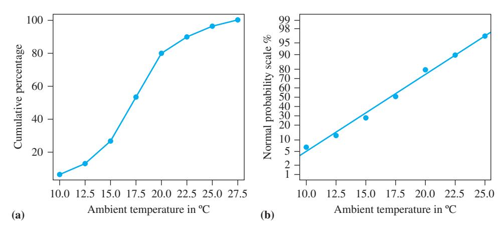
图 13.12 发动机 A 的累积百分比图:(a) 线性刻度;(b) 正态刻度。

图 13.12 可以通过以下 R 代码生成:
我们首先求出频率分布 breaks = c(0, 10, 12.5, 15, 17.5, 20, 22.5, 25, 27.5) temp_A_cut = cut(temp_A, breaks, right=FALSE) temp_A_freq = table(temp_A_cut) temp_A_freq # 然后我们用 cumsum 计算累积频率 cumfreq_A = 100*c(0, cumsum(temp_A_freq))/length(temp_A) plot(breaks[-1], cumfreq_A[-1], pch=19, cex=1.5, cex.lab=1.2, xaxt="n", yaxt="n", col="blue", main="", xlab=expression(paste('Ambient temperature in', ~degree,'C',sep='')), ylab="Cumulative percentage") axis(side = 1, at = seq(10, 27.5, by = 2.5)) axis(side = 2, at = seq(0, 100, by = 20), las = 1) # 连接各点 lines(breaks[-1], cumfreq_A[-1], lwd=2, col="blue") # 正态刻度上的累积百分比图 y <- qnorm(cumfreq_A/100) x <- breaks[-c(1,9)] y <- y[-c(1,9)]